Introduction
Working with human movement data, sometimes you need to make visualizations or infographics based on the data: you can better analyze the movement by visualizing it and its features see this, or maybe you just want to tell a story using movement visualizations.
Among different techniques for recording movement data, motion capture (mocap) is a well-known method for capturing the exact movements of an actor. Motion capture data are typically constructed from the 3D coordinates of body joints for a series of time-steps (frames). Mocap is often used to create animations for video games or feature films.
In a way, we can treat a segment of movement data like any tabular data: we have a sequence of frames (rows), and for each frame, we have the positions or rotations of a group of body joints (columns). However, there is a pre-defined spatial relationship among the body joints, which is the skeleton. We can use the skeleton to display not only the joints but also use the information of which joints are connected to each other to visualize the bones.
A great tool for creating web-based and interactive data-driven visualizations is the D3.js library. D3 allows you to create and manipulate web elements (the elements used in SVG, HTML, …) based on data. In addition, you can add transformations, transitions, and interactions to the visualizations using both D3 and the standard web practices that are available on modern web browsers.
In this post, you will learn how to read the parsed motion capture in javascript, and use D3.js to visualize the joints and bones in the skeleton. This is the first post in a series of posts, in which I’ll explain how to create more interesting visualizations based on movement and various features that we can extract from the movements of an actor.
Motion Capture Data Format
Mocap data are provided in different formats such as C3D (3D marker positions); Acclaim, Biovision, and Vicon (both the skeleton and the movement data); text (comma or space delimited); and more general 3D asset formats such as COLLADA.
No matter of the file formats, each frame of motion capture data consists of a root node, which defines the body’s absolute position and orientation with respect to a global coordinate system, and a set of nodes each representing a joint’s angle or bone’s relative orientation in a three-dimensional space.
For this guide, to avoid dealing with format-specific considerations and the mechanics of parsing them, I have provided sample mocap files in JSON format, available from the GitHub repository for this tutorial.
In our ad hoc format, we use two structures: one which contains the position of each joint at each time frame, and one for defining the skeleton (that is, the bones).
The positions are defined using an N x M matrix, representing N frames, each containing M joint objects. The position of each joint is defined by its three parameters x, y, and z. So, positions[0][4].x represents the position of the 5th joint along the x axis, at the first frame, and positions[99][14].z represents the position of the 15th joint along the z axis.
The skeleton is defined using an array of bones. Each element of the array contains two elements, representing the indexes of the two joint at each end of the bone. The indexes match the index of the joints as they appear in the positions matrix. For example, skeleton[0] = [6,7] represents the first bone in the skeleton, connecting the joint with index 6 (skeleton[0][0] = 6 to the joint with index 7(skeleton[0][1] = 7).
Setting Up the Scene
Before we start, we should include the D3.js and jQuery scripts in our HTML file:
We also need to create a div tag to put our visualization inside of it:
There are a number of variables and parameters that we are going to use throughout or project:
// Variables
var skeleton; // Storing the skeleton data
var positions;  // Storing the joint positions
var positions_scaled;  // Storing the scaled joint positions
var figureScale = 2;  // The scaling factor for our visualizations
var h = 200;  // The height of the visualization
var w = 400;  // The width of the visualization
We will put all of the code for doing the visualization inside of the draw() function.
function draw() {

}
Reading Mocap Data in Javascript
Our data is already in JSON format and ready to be used. We can use jQuery (or any other method of choice) to download and parse them:
// Read the files
$.getJSON("Skeleton_BEA.json", function(json) {
    skeleton = json;
    $.getJSON("BEA1.json", function(json) {
        positions = json;
        draw();
    });
});
Since the $.getJSON() function is asynchronous, we can only start drawing once all the data is loaded. Thus, we put all of the visualization code inside the draw() function and call it in the callback function of the last JSON file. Once the draw() function is called, we can access the data using the positions and skeleton global variables.
Setting Up the Environment
First, we create the SVG tag inside of our container, which will house all of the elements we visualize:
var parent = d3.select("body").select("#container");

var svg = parent.append("svg")
                .attr("width", w)
                .attr("height", h)
                .attr("overflow","scroll")
                .style("display","inline-block");
Before visualizing the data, we need to scale and translate them to make sure they are within a range that fits our intended design.
// Scale the data
positions_scaled = positions.map(function(f, j) {
    return f.map(function(d, i) {
      return {
        x: (d.x + 50) * figureScale,
        y: -1 * d.y * figureScale + h - 10,
        z: d.z * figureScale
      };
    });
  });
Note that the y axis in motion capture data start from the bottom of the screen, while D3 expects the y axis to start from the top. Thus, we need to multiply it by -1 and translate it by the hight of our container.
We start by drawing the pose of only one frame, identified by the index variable.
// Choose the frame to draw
index = 60;  // the index of the frame
currentFrame = positions_scaled[index];
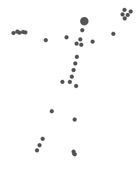
Visualizing the Joints
We visualize joints with circles. Based on the data from the currentFrame, we append an SVG circle element for each joint and set its center to the position of the joint. We further specify the radius of the circles and their filling color. We can make specific joints bigger, or paint them with a different color, by checking the index i passed to the function function(d,i).
headJoint = 7;

svg.selectAll("circle.joints" + index)
.data(currentFrame)
.enter()
.append("circle")
.attr("cx", function(d) {
    return d.x;
}).attr("cy", function(d) {
    return d.y;
}).attr("r", function(d, i) {
    if (i == headJoint )
        return 4;
    else
        return 2;
}).attr("fill", function(d, i) {
    return '#555555';
});
The code above will give you this:
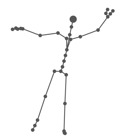
Adding the Bones
We visualize each bone with a line connecting the two joints at each end. We use the skeleton array as our main data source. For each bone, we add an SVG line element. The locations of the beginning and the end of the line is determined by the positions of the first and second joints of the bone. Note that the position data are stored in the currentFrame variable:
 svg.selectAll("line.bones" + index)
.data(skeleton)
.enter()
.append("line")
.attr("stroke", "#555555")
.attr("stroke-width",1)
.attr("x1",0).attr("x2",0)
.attr("x1", function(d, j) {
    return currentFrame[d[0]].x;
})
.attr("x2", function(d, j) {
    return currentFrame[d[1]].x;
})
.attr("y1", function(d, j) {
    return currentFrame[d[0]].y;
})
.attr("y2", function(d, j) {
    return currentFrame[d[1]].y;
});
Now, your visualization should look like this:
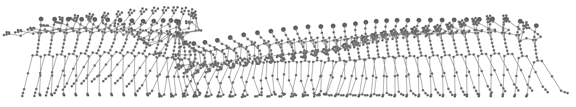
Drawing More Frames
So far we have only visualized a single frame. Now, we go one step further and draw a sequence of consecutive frames.
We use two more parameters. The distance between each two consecutive frames will be defined by the gap variable. Also, we may not necessarily want to draw every single frame and instead only draw every 4th frame (downsampling). We specify this fraction by the skip variable.
var gap = 20; // in pixels
var skip = 20; // number of frames to skip
We visualize a sequence of frames by applying the D3 functions on a nested datasource. First, we apply a filter on the positions_scaled array to skip the frames we don't want to draw:
positions_scaled.filter(function(d, i) {
    return i % skip == 0;
})
Next, we loop through the frames, and append the elements for the data for each frame. We create an SVG group element for each frame and shift its position by the pixels specified in gap:
.append("g")
.attr("transform",function(d,i) {
    return "translate("+(i*gap)+",0)";
})
We then add the joints or bones inside of this SVG group element.
// Joints
svg.selectAll("g")
    .data(positions_scaled.filter(function(d, i) {
        return i % skip == 0;
    }))
    .enter()
    .append("g")
    .attr("transform",function(d,i) {
                return "translate("+(i*gap)+",0)";
    })
    .selectAll("circle.joints")
    .data(function(d,i) {return d})
    .enter()
    .append("circle")
    .attr("fill-opacity","0.95")
    .attr("cx", function(d) {
    return d.x;
    }).attr("cy", function(d) {
    return d.y;
    }).attr("r", function(d, i) {
    if (i == headJoint)
        return 4;
    else
        return 2;
    }).attr("fill", function(d, i) {
    return '#555555';
    });

// Bones
svg.selectAll("g2")
    .data(positions_scaled.filter(function(d, i) {
        return i % skip == 0;
    }))
    .enter()
    .append("g")
    .attr("transform",function(d,i) {
                return "translate("+(i*gap)+",0)";
    })
    .selectAll("line.bones")
    .data(skeleton)
    .enter()
    .append("line")
    .attr("stroke-opacity","0.95")
    .attr("stroke", "grey")
    .attr("stroke-width", 1)
    .attr("x1", 0).attr("x2", 0)
    .attr("x1", function(d, j, k) {
    return positions_scaled[k * skip][d[0]].x;
    })
    .attr("x2", function(d, j, k) {
    return positions_scaled[k * skip][d[1]].x;
    })
    .attr("y1", function(d, j, k) {
    return positions_scaled[k * skip][d[0]].y;
    })
    .attr("y2", function(d, j, k) {
    return positions_scaled[k * skip][d[1]].y;
    });
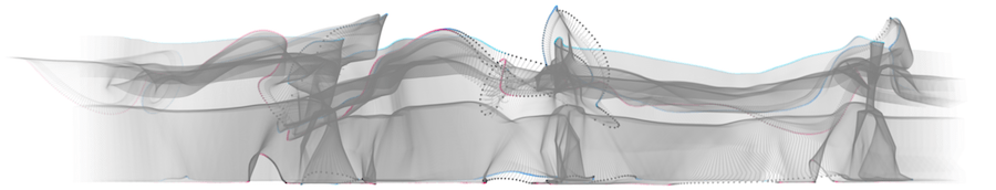
Now, you should be able to see this:
That's it for the first part of this tutorial. In the following posts, I will explain how to extract movement features and incorporate them into the visualizations.
The Complete Code
You can see the demos in action here and here.
The complete source code and data are in the github repo: https://github.com/omimo/d3-mocap-demo.
You can also play around with the code using this fiddle:
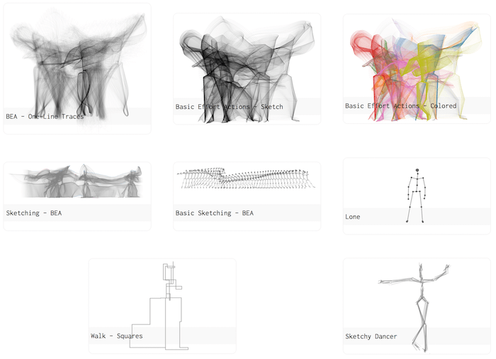
More Examples
If you are interested, you can take a look at more examples in the link below:
Further Resources
-
If you are interested in learning more about D3.js, you can find many tutorials here: https://github.com/d3/d3/wiki/Tutorials
-
To learn more about motion capture formats, here are some useful links:
Comments